Now that you have a basic understanding of the Fourier transform and some of the practical matters that arise from digital signals, it's time to look at a basic imaging pulse sequence and even make some simple images. We're going to use frequency encoding only for the time being, and for now we're going to make one-dimensional images (also called profiles) so that we can introduce an alternative form of timing diagram to represent a pulse sequence.
A magnetic field gradient alters the local resonance frequency
When a sample is placed into the magnet, all the protons (1-H nuclei) resonate at a near-identical frequency. At 3 T that resonance frequency is approximately 123 MHz, as given by the Larmor equation. If we then impose a magnetic field gradient across the sample - your subject's head, say - instead of having the same resonance frequency uniformly across the brain, there will now be a linear dependence in space (see Note 1):

In a real image we might consider 64 different positions along x. These would define the voxels in one (in-plane) dimension of the image. But for the time being we'll consider just three points in the x direction: the central point, and one point either side.
At the center of the magnet the gradient has no net effect, so the resonance frequency at that point is still 123 MHz. We call this point the null crossing, because all three linear gradients, X, Y and Z, are engineered to have no effect here. (See Note 2.) And to keep things symmetric, the gradient null crossing is placed in the geometric center of the magnet - the isocenter - because that's where the main magnetic field has been engineered to be most homogeneous, and we want to do all our imaging in that location to get the best scanner performance.
At the magnet isocenter, then, the resonance frequency is left unchanged by Gx. Otherwise, the resonance frequency is now x-dependent according to:
At the magnet isocenter, then, the resonance frequency is left unchanged by Gx. Otherwise, the resonance frequency is now x-dependent according to:

At isocenter the sample experiences exactly 3 T whereas to the left of center (at position x1) the sample is at a field slightly less than 3 T (there's partial cancellation where the gradient field opposes the main magnetic field), and to the right of center (at x2) it's at a magnetic field slightly greater than 3 T. (See Note 3.) The spatial dependence of the resonance frequency is linear. (If you think I'm doing an obvious point to death, take a look at Note 4.)

We can simplify the representation a little by considering a rotating reference frame, rather than the static reference frame of the magnet (which is known as the laboratory frame). We deal with a rotating frame all the time. Hands up who navigates relative to static positions on the earth? We conveniently discount the fact that we're rotating at a thousand miles an hour about the earth's axis, or that the earth is rotating about the sun, etc. Likewise, in MRI we take a reference rotational frequency - the nominal resonance frequency at the center of the magnet, which is 123 MHz here - and we then consider frequencies slightly faster or slower than the reference. These frequency differences manifest as phase shifts for the spins in the rotating frame picture. (See Note 5.)
Below left, I've represented the resonance frequencies for three chunks of magnetization, one located at isocenter and one each for positions x1 and x2, relative to the Gx gradient illustrated above. In this vector diagram, equilibrium magnetization (before RF excitation) would be indicated by a vertical arrow pointed along the +z axis; all three chunks of magnetization would reside there. But after RF excitation, and following the imposition of the gradient Gx, the magnetization will be spread out and there will be local differences in resonance frequency, depending on position x:
 |
| LEFT: Magnetization in the rotating reference frame for three positions along x after imposition of a gradient Gx. RIGHT: The resonance frequencies in the lab frame (white) and in the rotating frame (colors) for the three positions. |
In general then, the spatially-dependent frequency is given by:

Acquiring an MR signal in the presence of a gradient
Achieving the situation you've just encountered can be represented on a timing diagram, such as this one:

Starting with equilibrium magnetization (which isn't indicated, just assumed), a 90 degree RF excitation pulse rotates all proton spins in the sample from the z axis into the transverse plane of the rotating reference frame. The gradient, Gx is then activated, differentiating resonance frequencies with an x spatial dependence as we just saw. (See Note 6.) There's also T2 relaxation going on, but we will be able to ignore this for the purposes of spatial encoding; I include it below purely to show how the effect of the gradient and the innate relaxation have similar mathematical representations. Provided the decaying magnetization persists for enough time to record it - with our analog-to-digital converter, ADC - we're in good shape. (See Note 7.)
In the absence of a gradient, the transverse magnetization decays with T2 relaxation only:

where Mxy(t=0) is the magnetization immediately after the 90 degree excitation pulse.
If we turn on a gradient after the excitation pulse then there is an additional dephasing, resulting in further attenuation of net magnetization as well as providing the desired spatial encoding:
Spatial information is encoded because, as we've seen above, frequency (w) is a function of position, x when Gx is turned on. The term in yellow, arising from the gradient we've enabled, is just another dephasing term, albeit one that now contains some useful spatially-dependent information. (See Note 8.)
Now all we have to do is "decode" the spatial information resident in the yellow exponent. This can be accomplished quite simply by Fourier transformation of Mxy because, as we saw in Part Five, an FT will produce a one-dimensional plot of the frequency content of a time domain signal. If we ignore the T2 relaxation for simplicity (by assuming that it's very small during the gradient encoding and data acquisition period) then the signal intensity at each position along the one-dimensional frequency plot will be proportional to the spin density at that position, as represented by Mxy(t=0) in the equation above. Let's see this process in action.
We'll start with a cylinder filled with water so that the magnetization is uniform throughout, and zero outside. The x gradient will be applied perpendicular to the cylinder's axis:

The gradient creates a range of frequencies for each position, x across the cylinder's cross-section:

Next, we need to determine how much signal we will receive from each position along x, which we do with the Fourier transform. From the figure above let's suppose there are n=64 positions along x to consider. After FT the amount of signal in the frequency domain will be directly proportional to the spin density in each of the 64 planes orthogonal to the x direction. Clearly, at positions (such as x1 and x2 above) outside the sample there will be zero signal. Within the sample the spin density is uniform, but the shape of the cylinder means that each plane will 'sample' different volumes of water. The plane that samples the central section of the cylinder along x will obviously contain the highest number of protons (hence largest magnetization), thus will be the tallest portion of the frequency plot.
If we do this process 64 times and then join up the signal amplitudes in the frequency domain we end up with a one-dimensional image of the cross-section of the cylinder, as shown by the green ellipse below. I've indicated one plane, in red, through the cylinder to show the origin of the profile explicitly:

That was easy, right? Good. Then try two new samples on for size. Not only will we add a second water-filled sample having a trapezoidal cross-section, let's also measure a profile of the two objects along the y axis as well as x. For the y profile we'd do a separate experiment in which we apply a gradient, Gy instead of Gx. (See Note 9.)
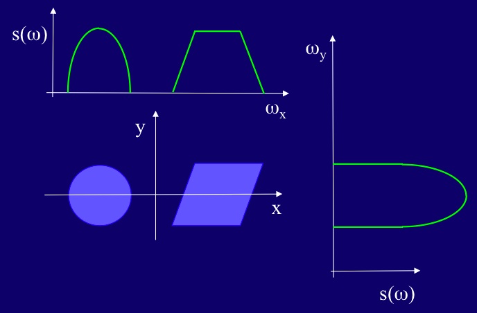
A final point for today. In the last example I didn't mention the length of the two objects being imaged. What would be the relative heights of the cylinder and the trapezoid? Well, if you assume the light blue color indicates equivalent spin density for the water in each shape then, given that the peak intensities in the x profiles are the same, we would have to conclude that the lengths are equivalent. (The total number of spins in a plane through the center of each sample is the same.) Had I drawn the cylinder's profile along x with, say, twice the maximum amplitude of the trapezoid's then you could have concluded that the cylinder were twice the length of the trapezoid (again assuming equal spin density). If the length of the cylinder had been twice the length of the trapezoid, what would the y profile have looked like...?
Next post: gradient-recalled echoes and slice selection. After that, two-dimensional imaging!
----------------------
Notes:
1. We abbreviate magnetic field gradient to gradient pervasively in fMRI. There are other gradients in MRI, depending on what you're doing (e.g. temperature gradients), but 99.9% of the time when an MRI person uses the term gradient a magnetic field gradient is assumed.
2. If you're curious what MRI gradient coils look like and how they work, there's a simple introduction in the book, "Functional Magnetic Resonance Imaging" by Huettel, Song and McCarthy. In the second edition it's on pages 38-40. Modern gradient coil designs have come a long way from the basic conceptual designs that you'll mostly find in books, however. Vendors treat their designs like state secrets, and with good reason. The majority of MRI physicists would probably agree that stable, high fidelity, high powered gradients are the most critical aspect of overall MRI performance. Perhaps I'll do a separate post on gradients at a later date. Unless you're responsible for specifying and buying a new MRI scanner, or you're charged with doing your center's QA, you really don't need to understand the engineering of the gradients in order to do fMRI experiments.
3. On a typical 3 T scanner the maximum magnetic field gradient amplitude is around 40 mT/m. So the gradients are three orders of magnitude smaller than the main magnetic field. You don't need a whole lot of magnetic field strength to encode spatial information!
4. In a nutshell, this is what Paul Lauterbur did in 1973 to get himself a Nobel Prize (awarded in 2003, jointly with Sir Peter Mansfield). Okay, so Lauterbur had to do a little more work than this – he imposed a series of gradients at different orientations relative to two tubes of water, then used a back-projection algorithm to compute a 2D image of the tubes – but a linear modification of the Larmor equation was, in essence, his crucial insight. And it’s pretty darn funny in hindsight - at least it is to a reformed spectroscopist like myself - because for the first thirty-odd years of NMR, from the first successful measurements by Bloch and Purcell in 1946, everybody had been working really hard to get the flattest, most homogeneous magnetic field possible. Then along comes Lauterbur, tilts the magnetic field so that it has a known (linear) spatial dependence, invents MRI and asks the receptionist if he might now have his Nobel Prize, please. No wonder Damadian was so ticked off.
Lest you should get despondent when your latest fMRI paper gets rejected, apparently Lauterbur ran into obstacles trying to patent his idea, and then had his first attempt to publish in Nature rejected. Ah, peer review. You have to laugh, don't you? Anyway, here's Lauterbur's image, the very first MRI:
5. The rotating reference frame, denoted by primes, rotates about the lab frame such that +z and +z' are parallel and aligned (by convention) along the main magnetic field direction, B0. In this representation the x and y lab axes are whirling around z at 123 MHz, rendering the rotation of the magnetization, and the rotating axes x' and y', static in this view. Then any precessional frequency changes of magnetization will appear as phase shifts relative to the (now static) x' and y' axes.
Lest you should get despondent when your latest fMRI paper gets rejected, apparently Lauterbur ran into obstacles trying to patent his idea, and then had his first attempt to publish in Nature rejected. Ah, peer review. You have to laugh, don't you? Anyway, here's Lauterbur's image, the very first MRI:
 |
| From: P.C. Lauterbur, Nature 242, 190-1 (1973). |
5. The rotating reference frame, denoted by primes, rotates about the lab frame such that +z and +z' are parallel and aligned (by convention) along the main magnetic field direction, B0. In this representation the x and y lab axes are whirling around z at 123 MHz, rendering the rotation of the magnetization, and the rotating axes x' and y', static in this view. Then any precessional frequency changes of magnetization will appear as phase shifts relative to the (now static) x' and y' axes.
6. On my magnet at least, the magnetic field gradients form a right-handed set. That is, if you hold up the index finger, middle finger and thumb of your right hand so that they are orthogonal, your index finger indicates +Z, the magnetic field direction (towards the front of the magnet), your middle finger indicates the +X direction, which is the subject's left (assuming the subject is in head first, supine), and your thumb indicates +Y, towards the top of the magnet.

7. If you are already familiar with pulse sequences then you will immediately spot the lack of a gradient-recalled echo, which is how we usually acquire MRI data for several experimental reasons, and it's T2* rather than T2 relaxation that's happening. I'm keeping it simple for now. Worry not, the GRE will be along in the next post. Likewise, I'm not using slice selection here because it's not necessary yet either. I want to get through the in-plane k-space representation first. We're going to go in the order: frequency encoding, phase encoding, slice selection.
8. I want to reinforce the point that the term in yellow, arising from the gradient we've enabled, is just another dephasing term. If we weren't interested in its spatial encoding properties (via the frequency distribution along x) then there is another "use" for this gradient pulse: it enhances signal attenuation. Furthermore, in MRI a gradient is a gradient is a gradient! Whether you are able to control it from the scanner console, as with Gx, or it arises intrinsically because of the properties of your sample (e.g. your subject's skull, or his blood vessels), the effect is the same as far as the spins are concerned. Really, the only differences between our linear gradients and the gradients that arise intrinsically is this aspect of control, the known (linear) spatial dependence of Gx,y,z, and the length over which the gradients act. Gx,y,z are imposed across the entire sample, whereas the subject's skull probably has quite local effects. Beyond these differences, however, the spins don't care. If they experience a gradient arising from the skull or from Gx they will dephase all the same. This is good and bad news; bad news because it will cause difficulties for image localization, good news because it creates this thing called BOLD and enables one version of fMRI. More on all of this stuff in many later posts.
9. Why can't we turn on Gx and Gy at the same time, and why must we acquire each profile in separate experiments? If Gx and Gy are on simultaneously we would then have one gradient that is the vector sum of Gx and Gy, not separate x and y gradients! The combined gradient would create another profile in a direction 45 degrees between x and y.
NO COMMENTS, C'MMON PEOPLE!
ReplyDeleteSeriously now, that's really a good paper. It keeps thing simple and helped me a lot. Thanks!
This is so helpful! I have been reading through all the physics for understanding posts and the fourier transform explanation as well as convolution made the things I learned as an undergrad SO much clearer. Several of the pictures across the various posts don't show and the videos don't work any more either FYI. Thanks again!
ReplyDeleteHi Ryan, glad you found it all useful! I just quickly clicked through the series and I don't see any places where the pix or videos don't show up properly. Which post(s) did you run into problems with?
Delete2023 and these posts are still helpful! thanks again for doing these
ReplyDelete