Education, tips and tricks to help you conduct better fMRI experiments.
Sure, you can try to fix it during data processing, but you're usually better off fixing the acquisition!

Friday, December 14, 2012

Inadequate fat suppression for diffusion imaging


Diffusion imaging is often included as a component of functional neuroimaging protocols these days. While fMRI examines functional changes on the timescale of seconds to minutes, diffusion imaging is able to detect changes over weeks to years. Furthermore, there may be complimentary information from the white matter connectivity obtainable from diffusion imaging – that is, from tractography - and the functional connectivity of gray matter regions that can be derived from resting state or task-based fMRI experiments.

I was recently made aware of some artifacts on diffusion-weighted EPI scans acquired on a colleagues’ scanner. When I was able to replicate the issue on my own scanner, and even make the problem worse, it was time to do a serious investigation. The origin of the problem was finally confirmed after exhaustive checks involving the assistance of several engineers and scientists from Siemens. The conclusion isn't exactly a major surprise: fat suppression for diffusion-weighted imaging of brain is often insufficient. And it seems that although the need for good fat suppression is well known amongst physics types, it’s not common knowledge in the neuroscience community. What’s more, the definition of “sufficient” may vary from experiment to experiment and it may well be that numerous centers are unaware that they may have a problem.

Let’s start out by assessing a bad example of the problem. The diffusion-weighted images you’re about to see were acquired from a typical volunteer on a Siemens TIM/Trio using a 32-channel receive-only head coil, with b=3000 s/mm2 (see Note 1), 2 mm isotropic voxels, and GRAPPA with twofold (R=2) acceleration. These are three successive axial slices:


(Click to enlarge.)

The blue arrows mark hypointense artifacts whereas the orange arrow picks out a hyperintense artifact. Even my knowledge of neuroanatomy is sufficient to recognize that these crescents are not brain structures. They are actually fat signals, shifted up in the image plane from the scalp tissue at the back of the head. (If you look carefully you may be able to trace the entire outline of the scalp, including fat from around the eye sockets, all displaced anterior by a fixed amount.) I’ll discuss the mechanism later on, but at this point I’ll note that the two principal concerns are the b value (of 3000 s/mm2) and the use of a 32-channel array coil. GRAPPA isn’t a prime suspect for once!

Now, part of the problem is that the intensity of the artifacts – but not their location - changes as the direction of the diffusion-weighting gradients changes. In the following video you see the diffusion-weighted images as the diffusion gradient orientation is changed through thirty-two directions (see Note 2):


The signal from white matter fibers changes as the diffusion gradient direction changes. That’s what you want to happen. But the displaced fat artifacts also change intensity with diffusion gradient direction, meaning that the artifact is erroneously encoded as regions of anisotropic diffusion. Thus, when one computes the final diffusion model, the brain regions contaminated by fat artifacts end up looking like white matter tracts. In the next figure the data shown above was fit to a simple tensor model, from which a color-coded anisotropy map can be obtained:


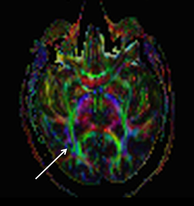
The white arrow picks out the false “tract” corresponding to the artifact signal crescent we saw on the raw diffusion-weighted images. I suppose it’s remotely possible that this is the iTract, a new fasciculus that has evolved to connect the subject’s ear to his smart phone, but my money is on the fat artifact explanation.

Clearly, in the above image there is no easy way to distinguish the artifact from real white matter tracts by eye, except by using your prior anatomical knowledge. And it's likely to confuse tractographic methods, too, because it has very similar geometric properties to those that tractographic methods attempt to trace. So let's take a look at the origin of the problem and then we can get into what you want: solutions. 

Saturday, December 1, 2012

Review: Differentiating BOLD from non-BOLD signals in fMRI time series using multi-echo EPI


Disclaimer: I'm afraid I haven't done a very good job reviewing the entirety of this paper because the stats/processing part was pretty much opaque to me. I've done my best to glean what I can out of it, and then I've focused as much as I can on the acquisition, since that is one part where I can penetrate the text and offer some useful commentary. Perhaps someone with better knowledge of stats/ICA/processing will review those sections elsewhere.


The last paper I reviewed used a bias field map to attempt to correct for some of the effects of subject motion in time series EPI. A different approach is taken by Prantik Kundu et al. in another recently published study. In their paper, Differentiating BOLD from non-BOLD signals in fMRI time series using multi-echo EPI, Kundu et al. set out to differentiate between signal changes that have a plausible neurally-driven BOLD origin from those that are likely to have been modulated by something other than neuronal activity. In the latter category we have cardiac and respiratory fluctuations and, of course, subject motion.

The method involves sorting BOLD-like from spurious changes using an independent component analysis (ICA) and to then "de-noise" the time series before applying connectivity analysis. For resting state fMRI in particular, the lack of any sort of ground truth and an absence of independent knowledge that one has with task-based fMRI makes disambiguating neurally driven signal changes from artifacts a major problem. Kundu et al. use a relatively simple philosophical approach to the separation:
"We hypothesized that if TE-dependence could be used to differentiate BOLD and non-BOLD signals, non-BOLD signal could be removed to denoise data without conventional noise modeling. To test this hypothesis, whole brain multi-echo data were acquired at 3 TEs and decomposed with Independent Components Analysis (ICA) after spatially concatenating data across space and TE. Components were analyzed for the degree to which their signal changes fit models for R2* and S0 change, and summary scores were developed to characterize each component as BOLD-like or not BOLD-like."

And, noting again the caveat that there is an absence of ground truth, the approach seems to work:
"These scores clearly differentiated BOLD-like “functional network” components from non BOLD-like components related to motion, pulsatility, and other nuisance effects. Using non BOLD-like component time courses as noise regressors dramatically improved seed-based correlation mapping by reducing the effects of high and low frequency non-BOLD fluctuations."

Wednesday, November 14, 2012

Review: Using a bias field map to improve motion correction of EPI time series


In a new paper entitled "Effects of image contrast on functional MRI image registration," Gonzalez-Castillo et al. evaluate the performance of motion correction (a.k.a. registration) following a pre-processing step that aims to remove the contrast imparted across images due to receive (and/or transmit) field heterogeneity. A bias field map is estimated from a target EPI, and this reference image is then used to normalize the other images in the time series. There are other aims in the paper, too: specifically, to evaluate the performance of image registration (EPI to EPI, or EPI to MP-RAGE anatomical) when the T1 contrast of time series EPIs is altered via the excitation RF flip angle. But in this post I am going to focus on the normalization part because it involves the RF receive field heterogeneity, and this instrumentally-induced contrast is of particular concern for exacerbating motion sensitivity in fMRI (as explained here).

Although others have compared prescan normalization between different array coils (see the references in this paper), this is the first paper I've seen that compares motion correction performance for EPI time series acquired with an array coil (a 16-channel array) to a single channel birdcage coil. Now, this isn't quite the straightforward comparison I might like - with the receive fields being the only difference - because in this instance the birdcage is also used to transmit the excitation RF pulses, making the transmission (Tx) field for the birdcage experiment more spatially heterogeneous than will be produced from the body RF coil that's used when acquiring with a receive-only array coil. Following? In other words, for the 16-channel array the receive (Rx) field heterogeneity is likely to dominate whereas for the birdcage coil the heterogeneities of both the transmit and receive fields are salient. Still, it's worth a look since the coil comparison highlights the issue of the scanner hardware's influence on EPI contrast, and on subsequent motion correction.

Saturday, October 27, 2012

Motion problems in fMRI: Receive field contrast effects


Motion has been identified as a pernicious artifact in resting-state connectivity studies in particular. What part might the scanner hardware play in exacerbating the effects of subject motion?


My colleague over at MathematiCal Neuroimaging has been busy doing simulations of the interaction between the image contrast imposed by the receiver coil (the so-called "head coil") and motion of a sample (the head) inside that coil. The effects are striking. Typical amounts of motion create signal amplitude changes that easily rival the BOLD signal changes, and spurious spatial correlations can be introduced in a time series of simulated data.

The issue of receive field contrast was recognized in a recent review article by Larry Wald:
"Highly parallel array coils and accelerated imaging cause some problems as well as the benefits discussed above. The most problematic issue is the increased sensitivity to motion. Part of the problem arises from the use of reference data or coil sensitivity maps taken at the beginning of the scan. Movement then leads to changing levels of residual aliasing in the time-series. A second issue derives from the spatially varying signal levels present in an array coil image. Even after perfect rigid-body alignment (motion correction), the signal time-course in a given brain structure will be modulated by the motion of that structure through the steep sensitivity gradient. Motion correction (prospective or retrospective) brings brain structures into alignment across the time-series but does not alter their intensity changes incurred from moving through the coil profiles of the fixed-position coils. This effect can be partially removed by regression of the residuals of the motion parameters; a step that has been shown to be very successful in removing nuisance variance in ultra-high field array coil data (Hutton et al., 2011). An improved strategy might be to model and remove the expected nuisance intensity changes using the motion parameters and the coil sensitivity map."

In our recent work we take a first step towards understanding the rank importance of the receive field contrast as it may introduce spurious correlations in fMRI data. It's early days, there are more simulations ongoing, and at this point we don't have much of anything to offer by way of solutions. But, as a first step we are able to show that receive field contrast is ignored at our peril. With luck, improved definition of the problem will lead to clever ways to separate instrumental effects from truly biological ones.

Anyway, if you're doing connectivity analysis or otherwise have an interest in resting-state fMRI in general, take a read of MathematiCal Neuroimaging's latest blog post and then peruse the paper submitted to arXiv, abstract below.

____________________


A Simulation of the Effects of Receive Field Contrast on Motion-Corrected EPI Time Series

D. Sheltraw, B. Inglis
The receive field of MRI imparts an image contrast which is spatially fixed relative to the receive coil. If motion correction is used to correct subject motion occurring during an EPI time series then the receiver contrast will effectively move relative to the subject and produce temporal modulations in the image amplitude. This effect, which we will call the RFC-MoCo effect, may have consequences in the analysis and interpretation of fMRI results. There are many potential causes of motion-related noise and systematic error in EPI time series and isolating the RFC-MoCo effect would be difficult. Therefore, we have undertaken a simulation of this effect to better understand its severity. The simulations examine this effect for a receive-only single-channel 16-leg birdcage coil and a receive-only 12-channel phased array. In particular we study: (1) The effect size; (2) Its consequences to the temporal correlations between signals arising at different spatial locations (spatial-temporal correlations) as is often calculated in resting state fMRI analyses; and (3) Its impact on the temporal signal-to-noise ratio of an EPI time series. We find that signal changes arising from the RFC-MoCo effect are likely to compete with BOLD (blood-oxygen-level-dependent) signal changes in the presence of significant motion, even under the assumption of perfect motion correction. Consequently, we find that the RFC-MoCo effect may lead to spurious temporal correlations across the image space, and that temporal SNR may be degraded with increasing motion.

Thursday, October 11, 2012

Draft checklist for fMRI methods reporting in the literature


It took a little longer to get to than I'd planned, but contained in this post is a first pass at a checklist for acquisition parameters that I think should be included in the methods section of fMRI papers. This draft is an attempt to expand and update the list that was given in the 2008 paper from Poldrack et al. (I have reproduced below the section on acquisition that appeared in that 2008 paper.) Here, I tried to focus on the bulk of fMRI experiments that use 1.5 to 3 T scanners with standard hardware today. I further assumed that you're reporting 2D multislice EPI or spiral scanning. Advanced and custom options, such as multiband EPI, 3D scans and 7 T, will have to be added down the road.

In an attempt to make it didactic I have included explanatory notes. I went verbose instead of shorthand on the assumption that many fMRI papers don't include a lot of experimental detail perhaps because the authors don't possess that level of knowledge. We might as well learn something new whilst satisfying our collective desire for better manuscripts, eh? So, I haven't even tried to determine a shorthand notation yet. As others have already commented, having a checklist is probably more useful in the near term and the idea of a shorthand is a secondary consideration that has most value only if/when a journal is attempting to curtail the length of methods sections. But I'll take a stab at a shorthand notation once the checklist has been refined in light of feedback.

I've sorted the parameters into Essential, Useful and Supplemental categories in terms of value to a reader of a typical fMRI paper. Within each category the parameters are loosely sorted by functional similarity. In the Essential category are parameters whose omission would challenge a reader's ability to comprehend the experiment. Thus, there are several acquisition options - sparse EPI for auditory stimulus delivery is one example - that appear under Essential even though they are rarely used. The assumption is that everyone would report all the Essential parameters, i.e. that a reviewer should be expected to fault a paper that doesn't contain all the Essential parameters (and a journal should be held accountable for not permitting inclusion of all Essential parameters in the published methods section rather than consigning them to supplemental material).

Friday, October 5, 2012

Next-gen platforms for evaluating scientific output


Tal Yarkoni has a paper out in Frontiers in Neuroscience, "Designing next-generation platforms for evaluating scientific output: what scientists can learn from the social web." As someone who has recently taken the plunge into 'pre-publication' submissions, I shall be interested to hear others' opinions on the manifold issues surrounding online publication, peer review, post-publication review, etc.

To be honest I'm a little surprised someone down in the South Bay (that's Silicon Valley to you non-Bay Area locals) hasn't already created a startup company offering us software to do this stuff. Surely there's money to be made. Until then, I for one have moved in toto to faster online models, whether it's this blog for my local user support (which just happens to take precisely the same amount of work whether fifty or fifty million people read it) or arXiv.org for papers. I'm adopting the Nike model: Just do it. But I realize it's a lot more complicated and nuanced than one rebellious Limey who already has a secure job. If we all went off piste there'd be chaos. So, how do we get from Tal's circumspect arguments to a workable platform?

Thursday, October 4, 2012

Introduction to MR principles: online resources


I recently came across some extremely informative online resources for learning the basics of (nuclear) magnetic resonance. The first (via Agilent's Spinsights.net blog) is an online simulator that is nicely introduced in a series of four YouTube tutorials (see below). The simulator allows you to demonstrate such concepts as RF excitation, the rotating frame of reference, relaxation and even a 1D gradient for spatial encoding. If you are brand new to MR then you might need some assistance in understanding things for yourself, and I would think this tool (and the supporting tutorials) would be best used by an instructor in a class, but I don't want to dissuade you from taking a stab on your own. Watch the videos first (see below), then check out the simulator. (You can also find technical info and links to the tutorials at www.drcmr.dk/bloch.)

The other resource I found just about blew me away, not so much for the NMR lectures themselves, as good as they are, but because they are part of an extensive biophysics course covering everything from electromagnetic radiation to flow cytometry and sedimentation methods! The lectures are by Yair Meiry, a fellow who is apparently now working as a skydiving instructor in Canada (assuming my Internet sleuthing has improved since yesterday's attempt to divine the Scandinavian country of origin of another YouTube video). Channeling his inner Garrett Lisi, perhaps? I know I'm impressed.

Wednesday, October 3, 2012

Quench!!!

I was persuaded by Tobias Gilk to post a video of the quench of Berkeley's old 4 T magnet, a fairly momentous event that a lot of people have enjoyed watching in private (whether they were absent or witnessed it live). The quench happened back in 2009. We didn't publicize the video at the time because we didn't want a bunch of know-nothings accusing us of wasting resources. (See the FAQ in the video comments if you want to know what happened to the magnet - we turned it into a mock scanner - and why we didn't try to recover the helium.) But there comes a time when the value to others becomes greater than the annoyance of poorly informed trolls venting their spleens on YouTube. So here it is, finally:


In case you missed seeing some of our antics in the couple of days leading up to the quench, here's that video, too:


And finally, while uploading the most recent video I tripped over another quench video from what looks and sounds like some Scandinavians: (I'm not even going to guess between Finland, Denmark, Norway, Sweden, Iceland,...)


Looks like these guys had as much fun as we did! What's really clear in their tests is the oscillation of magnetic objects between the regions of peak gradient at either end of the magnet - a couple of feet out from the faces of the magnet at either end, the magnetic field and cryostat being symmetrical. The speed of movement is sufficiently slow at 1.5 T to see things clearly, versus the crazy violent movement of objects in the 4 T field. They have better music, too.

Tuesday, October 2, 2012

We're arXiving! (Another post on GRAPPA.)


In another move to accelerate the development of methods for neuroimaging applications, some colleagues and I recently decided to abandon a second attempt to publish a paper in traditional journals and opted for the immediacy of arXiv instead. (Damn, it feels good to be free of reviewers claiming "What problem? I don't see why a solution is even needed?" Whatever.) We've got another paper coming out on arXiv in a few days, too, although in this case we are exploring the possibility of a simultaneous submission to IEEE Trans Med Physics since it allows such tactics, and my colleagues in "real" physics do this all the time. Whether or not the IEEE submission happens the material will be out there in the world, naked, for all to view and poke at. Isn't this how science is supposed to work? I love it!

Anyway, for today, here's the skinny on the arXiv submission from August (which I inadvertently forgot to hawk on this blog even after tweeting it):

http://arxiv.org/abs/1208.0972

(Get a PDF fo' free via the link.)


Simultaneous Reduction of Two Common Autocalibration Errors in GRAPPA EPI Time Series Data
 
D. Sheltraw, B. Inglis, V. Deshpande, M. Trumpis *
The GRAPPA (GeneRalized Autocalibrating Partially Parallel Acquisitions) method of parallel MRI makes use of an autocalibration scan (ACS) to determine a set of synthesis coefficients to be used in the image reconstruction. For EPI time series the ACS data is usually acquired once prior to the time series. In this case the interleaved R-shot EPI trajectory, where R is the GRAPPA reduction factor, offers advantages which we justify from a theoretical and experimental perspective. Unfortunately, interleaved R-shot ACS can be corrupted due to perturbations to the signal (such as direct and indirect motion effects) occurring between the shots, and these perturbations may lead to artifacts in GRAPPA-reconstructed images. Consequently we also present a method of acquiring interleaved ACS data in a manner which can reduce the effects of inter-shot signal perturbations. This method makes use of the phase correction data, conveniently a part of many standard EPI sequences, to assess the signal perturbations between the segments of R-shot EPI ACS scans. The phase correction scans serve as navigator echoes, or more accurately a perturbation-sensitive signal, to which a root-mean-square deviation perturbation metric is applied for the determination of the best available complete ACS data set among multiple complete sets of ACS data acquired prior to the EPI time series. This best set (assumed to be that with the smallest valued perturbation metric) is used in the GRAPPA autocalibration algorithm, thereby permitting considerable improvement in both image quality and temporal signal-to-noise ratio of the subsequent EPI time series at the expense of a small increase in overall acquisition time.


* For some strange arXiv technical reason the author list is reordered from that which appears (correctly) on the PDF. C'est la vie.

Wednesday, September 19, 2012

Understanding fMRI artifacts: CONTENTS


An organizational post I'd been meaning to get to for a while. There are some posts to come in this series, in parentheses below. I'll update this page with links as these posts get published.


Understanding fMRI artifacts

An introduction to the post series, defining what we mean by "good" data, and general discussion on viewing and interpreting EPI artifacts in a time series.


Good data


Understanding fMRI artifacts: "Good" axial data

Includes cine loops through time series EPI and statistical images to evaluate the data.


Understanding fMRI artifacts: "Good" coronal and sagittal data

Includes cine loops through time series EPI and statistical images to evaluate the data. (The notes include a description of the slice-dependent gradient switching limits that can prohibit certain slice orientations.)


Common persistent EPI artifacts


Common persistent EPI artifacts: Aliasing, or wraparound

Aliasing effects in the frequency and phase encoding dimensions.


Common persistent EPI artifacts: Gibbs artifact, or ringing

The origin of the ringing problem and demonstrations in phantom and brain data.


Common persistent EPI artifacts: Abnormally high N/2 ghosts (1/2)

Tuesday, September 11, 2012

Intense stray (static) magnetic field gradients may affect cognition


Have you ever wondered whether it's appropriate to put a research subject into a dark, confined tube that makes an awful din, whereupon the subject may learn that his brain has some abnormality, and still expect the subject's brain to operate in a state representative of his normal cognition (and not that of a stressed out basket-case)? And what about the bioeffects of the high magnetic field itself, or of the rapidly switched gradients and their induced electric currents in body tissue? To date there has been scant evidence that the action of studying human cognition via an MRI scanner actually modifies that brain function in a manner that might be considered a significant issue for interpretation of fMRI results.

Putting aside the cognitive effects of a loud background noise and claustrophobia, the question remains whether the static and time-varying magnetic fields are modifying brain function in a substantial fashion. There are some well-known side effects of high magnetic fields: vertigo (see Note 1), and a metallic taste are the two phenomena tied directly to presence of, or movement through, a high magnetic field. (See Note 2.) But these effects tend to be mild and/or transitory, as a subject acclimatizes to the magnetic field, and can usually be rendered negligible by taking care not to make rapid head movements in or around the magnet.

A colleague forwarded to me yesterday a paper from a Dutch group (van Nierop et al., "Effects of magnetic stray fields from a 7 tesla MRI scanner on neurocognition: a double-blind randomized crossover study." Occup. Environ. Med. 2012 Epub) that investigates the effects of head movements in the intense stray field region of a 7 T magnet. So, first of all, some good news: if you're doing fMRI at 1.5 or 3 T and you're not in the habit of asking your subjects to thrash their heads around wildly at the mouth of the magnet or once inside the magnet bore, then so far as is known today you're in the clear. The effects reported in this paper pertain specifically to head movement in the really intense gradients that comprise the stray magnetic field around the outside of a passively shielded 7 T magnet. (The iron shield is outside the magnet, leaving considerable gradients in the vicinity of the magnet when compared to the actively shielded 1.5 and 3 T magnets most of us have nowadays.)

And with that preamble let's look at the summary of the paper:


OBJECTIVE:  This study characterises neurocognitive domains that are affected by movement-induced time-varying magnetic fields (TVMF) within a static magnetic stray field (SMF) of a 7 Tesla (T) MRI scanner.

METHODS:  Using a double-blind randomised crossover design, 31 healthy volunteers were tested in a sham (0 T), low (0.5 T) and high (1.0 T) SMF exposure condition. Standardised head movements were made before every neurocognitive task to induce TVMF.

RESULTS:  Of the six tested neurocognitive domains, we demonstrated that attention and concentration were negatively affected when exposed to TVMF within an SMF (varying from 5.0% to 21.1% per Tesla exposure, p<0.05), particular in situations were high working memory performance was required. In addition, visuospatial orientation was affected after exposure (46.7% per Tesla exposure, p=0.05).

CONCLUSION:  Neurocognitive functioning is modulated when exposed to movement-induced TVMF within an SMF of a 7 T MRI scanner. Domains that were affected include attention/concentration and visuospatial orientation. Further studies are needed to better understand the mechanisms and possible practical safety and health implications of these acute neurocognitive effects.


Okay, so let's make sure we're clear that although the test magnetic field strengths mentioned are 0.5 and 1.0 T, this refers to two heterogeneous regions of a stray magnetic field on the outside of a 7 T magnet:


Wednesday, September 5, 2012

i-fMRI: Prospective motion correction for fMRI?


An ideal fMRI scanner might have the ability to update some scan parameters on-the-fly, in order to reduce or eliminate the effects of subject motion. Today, this approach is commonly referred to as "prospective motion correction" because the idea is to adapt the acquisition so that (some of) the effects of motion aren't recorded in the data, in contrast to the routinely employed retrospective motion correction schemes, such as an affine registration algorithm applied during post-processing; that is, in between the acquisition and the stats/modeling, which can lead some people to refer to such steps as "pre-processing" if you have a stats/modeling-centric view of the fMRI pipeline.

On the face of it, ameliorating motion effects by not permitting them to be recorded in the time series data is a wonderful idea. Indeed, as the subtitle to this blog attests, I am a huge fan of fixes applied during the acquisition rather than waiting until afterwards to try to post-process away unwanted effects. But this preference assumes that any method actually works, and works robustly, in everyday use. For sure there will be limitations and compromises, yet the central question is whether the benefits outweigh the costs. In the specific case of prospective motion correction, then, does a scheme (a) eliminate the need to use retrospective motion correction, and (b) does it reduce the effects of motion without bizarre failure modes that can't be predicted or circumvented easily?

A good place to begin evaluating prospective motion correction schemes - indeed, all motion correction schemes - is to first asses their vulnerabilities. It's no good if the act of fixing one part of the acquisition introduces an instability elsewhere. Failure modes should be benign. Below, I list the major hurdles for motion correction schemes to overcome, then I consider how elaborate any solutions might need to be. The goal is to decide whether - or when - prospective motion correction can be considered better than the alternative (default) approach of trying to limit all subject motion, and deal with the consequences in post-processing.


What do we mean by motion correction anyway?

As conducted today, motion correction applied during post-processing generally refers to an affine or sometimes a non-linear registration algorithm that seeks to maintain a constant anatomical content in a stack of slices throughout a time series acquisition. Prospective motion correction generally refers to the same goal: conserving the anatomical content over time. But, as is well known, there are concomitant changes in the imaging signal, and perhaps the noise, when a head moves inside the magnet. Other signal changes that are driven by motion may remain in the time series data after "correction." Indeed, depending on the cost function being used, the performance of the motion correction algorithm to maintain constant anatomy over time may be compromised by these concomitant modulations.

Now, we obviously want to try to maintain the anatomical content of a particular voxel constant through time or we have a big problem for analysis! But as a goal we should use a more restrictive definition for an ideal motion correction method: after correction we seek the elimination of all motion-driven signal (and noise) modulations. The only signal changes remaining should be neurally-driven BOLD changes (if we're using BOLD contrast, which I assume in this post) and "physiologic noise" that isn't strongly coupled to head (skull) motion. (Accounting for physiologic noise is usually treated separately. That's the assumption I'll use in this post, although at a very fine spatial scale it's clear that physiologic noise is another form of motion sensitivity.)


Motion sensitivities in fMRI experiments

A useful first task is to consider all the substantial signal changes in a time series acquisition that can be driven by subject motion. What signal changes are concomitant with changes of anatomical content as the brain moves relative to the imaging volume? How complicated is this motion sensitivity? What aspects of the signal changes will require hardware upgrades to the scanner, and/or pulse sequence modifications in order to negate them? And are these capabilities already designed into a modern scanner or will they require substantial re-design? These are the questions to keep in mind as we review the major motion sensitivities.

Thursday, July 26, 2012

Methods reporting in the fMRI literature


(Thanks to Micah Allen for the original Tweet and to Craig Bennett for the Retweet.)


If you do fMRI you should read this paper by Joshua Carp asap:

"The secret lives of experiments: Methods reporting in the fMRI literature."

It's a fascinating and sometimes troubling view of fMRI as a scientific method. Doubtless there will be many reviews of this paper and hopefully a few suggestions of ways to improve our lot. I'm hoping other bloggers take a stab at it, especially on the post-processing and stats/modeling issues.

At the end the author suggests adopting some sort of new reporting structure. I concur. We have many variables for sure, but not an infinite number. With a little thought we could devise a simple, logical reporting structure that could be decoded by a reader just like a header can be interpreted from a headed file. (Dicom and numerous other file types manage it, you'd think we could do it too!)

To get things started I propose a shorthand notation for the acquisition side of the methods; this is the only part I'm intimately involved with. All we need to do is make an exhaustive list of the parameters and sequence options that can be used for fMRI, then sort them into a logical order and decide on how to encode each one. Thus, if I am doing single-shot EPI on a 3 T Siemens TIM/Trio with a 12-channel receive-only head coil, 150 volumes, two dummy scans, a TR of 2000 ms, TE of 30 ms, 30 descending 3 mm slices with 10% gap, echo spacing 0.50 ms, 22 degrees axial-coronal prescription, FOV 22.4x22.4 cm, 64x64 matrix, etc. then I might have a reporting string that looks something like this:

3T/SIEM/TRIO/VB17/12CH/TR2000/TE30/150V/2DS/30SLD/THK3/GAP0.3/ESP050/22AXCOR/FOV224x224/MAT64x64

Interleaved or ascending slices? Well, SLI or SLA, of course! 

Next we add in options for parallel imaging, then options for inline motion correction such as PACE, and extend the string until we have exhausted all the options that Siemens has to offer for EPI. All the information is available from the scanner, much of it is included in the data header.

But that's just the first pass. Now we consider a GE running spiral, then we consider a GE running SENSE-EPI, then a Philips running SENSE-EPI, etc. Sure, it's a teeny bit involved but I'm pretty sure it wouldn't take a whole lot of work to collect all the information used in 99% of the fMRI studies out there. Some of the stuff that could be included is rarely if ever reported, so we could actually be doing a whole lot better than even the most thorough methods sections today. Did you notice how I included the software version in my Siemens string example above? VB17? I could even include the specific type of shimming routine used, even the number and type of shim coils!

If an option is unused then it is simply included with a blank entry: /-/ And if we include a few well-positioned blanks in the sequence for future development then we can insert some options and append those we can't envisage today. With sufficient thought we could encapsulate everything that is required to replicate a study in a few lines of text in a process that should see us through the next several years. (We just review and revise the reporting structure periodically, and we naturally include a version number at the very start so that we immediately know what we're looking at!)

There, that's my contribution to the common good for today. I just made up a silly syntax by way of example. The precise separators, use of decimal points, etc. would have to be thrashed out. But if this effort has legs then count me in as a willing participant in capturing the acquisition side of this business. We clearly need to do better for a litany of reasons. One of them is purely selfish: I find it hard or impossible to evaluate many fMRI papers for wont of just a few key parameters. I think we can fix that. We really don't have an excuse not to.


i-fMRI: Introducing a new post series


My colleague, MathematiCal Neuroimaging and I have been discussing what we see as flaws or limitations in current functional MRI scanners and methods, and what the future might look like were there ways to change things. So, in part to force us to consider each limitation with more rigor, and in part to stimulate thought and even activity within the neuroimaging community towards a brighter future, we decided to start a new series of posts that we'll cross-reference on our blogs. This blog will focus on the hand-wavy, conceptual side of things while at MathematiCal Neuroimaging you'll find the formal details and the mathematics.

We have loose plans at the moment to address the following topics: magnetic field strength considerations, gradient coil design considerations, RF coil design considerations, pulse sequences, contrast mechanisms, and motion and motion correction. We're going to hit a topic based on our developing interests and the issues that our local user community brings to us, so apologies if your fave doesn't actually appear in a post for months or years to come.


"You wanna go where? I wouldn't start from here, mate."

Blogs seem like the perfect vehicle for idle speculation about a fantasy future. The issues and limitations are very real, however, so that's where we will initiate the discussions. Then, wherever possible, we will gladly speculate on potential solutions and offer our opinions on the solutions that seem apparent today. But we're not going to try to predict the future; we will invariably be wrong. That would also be beside the point. What we want to do is motivate researchers, engineers and scanner vendors to consider the manifold ways an fMRI scanner and fMRI methods might evolve.

Note that in the last paragraph I referred specifically to an "fMRI scanner." A moment's consideration, however, reveals that most of the technology used for fMRI didn't arise out of dedicated efforts to produce a functional brain imager per se. Instead, we got lucky. Scanners are designed and built as clinical devices (worldwide sales in the hundreds to thousands) and not research tools for neuroscience (worldwide sales in the tens per year for pure research applications). A typical MRI scanner has compromises due to expense, size of subjects, stray magnetic field, applicability of methods to (paid) clinical markets, etc. Other forces are at work besides the quality and utility of fMRI. And these forces can be a mixed blessing.

Thus, part of the motivation for writing this post series is to provoke consideration of alternative current technologies; hardware or methods that exist right now but for whatever reason aren't available on the scanner you use for fMRI. Perhaps there are simple changes that can benefit fMRI applications even if these changes compromise a clinical application. For some facilities, like mine, that would be an acceptable trade.


What's in a name?

On this blog I'll use the moniker i-fMRI to label these op-ed posts. You can interpret the i however you like. Mathematicians might want to consider an imaginary scanner. Engineers might want to consider an impractical scanner. (This variant happens to be my preference.) Economists and business types might think of an inflationary fMRI scanner, because it's likely that the developments we seek will only drive the cost up, not down. And you neuroscientists? Well, we hope you'll consider your ideal fMRI scanner.

(Apple, if you're reading this - too late. We already sold the i-fMRI trademark to some company in China. Sorry.)

Friday, July 6, 2012

Siemens slice ordering

I've heard on the wind that there is still confusion or even a total lack of awareness of the change in slice ordering for interleaved slices when going from an odd number to an even number of slices, or vice versa. It makes a big difference for slice timing correction. So I though I'd post below a section from my user training guide/FAQ as a ready reference. Note that as far as I know this change in slice ordering is only an issue for Siemens scanners running VB15 or VB17 software, I can't comment on VD11 or other versions, and I haven't actually tested any scanner platform except a TIM Trio. Furthermore, it's only an issue if you're using interleaved slices. If anyone has additional information, especially if it conflicts with the situation posted here, then the field would probably appreciate a comment!

__________________


In what order does the scanner acquire EPI slices?

There are three options for slice ordering for EPI. To understand the ordering you first need to know the Siemens reference frame for the slice axis: the negative direction is [Right, Anterior, Foot] and the positive direction is [Left, Posterior, Head]. The modes are then:
  • Ascending - In this mode, slices are acquired from the negative direction to the positive direction.
  • Descending - In this mode, slices are acquired from the positive direction to the negative direction.
  • Interleaved - In this mode, the order of acquisition depends on the number of slices acquired:
    • If there is an odd number of slices, say 27, the slices will be collected as:
1 3 5 7 9 11 13 15 17 19 21 23 25 27 2 4 6 8 10 12 14 16 18 20 22 24 26.
    • If there is an even number of slices (say 28) the slices will be collected as:
2 4 6 8 10 12 14 16 18 20 22 24 26 28 1 3 5 7 9 11 13 15 17 19 21 23 25 27.

Interleaved always goes in the negative to positive direction, e.g. foot-to-head for transverse slices.

So, if you are doing 28 interleaved axial slices the order will be evens then odds in the foot-to-head direction. 27 interleaved axial slices would also be acquired in the foot-to-head direction but would be in the order odds then evens. If you switch to 28 descending axial slices the acquisition order will become 1,2,3,4,5…28 and the direction will swap to being head-to-foot.

Tuesday, July 3, 2012

Physics for understanding fMRI artifacts: Part Thirteen

A tour through a real EPI pulse sequence

In some posts I've got planned it will be important for you to know something about all of the different functional modules that are included in a real EPI pulse sequence. So far in this PFUFA series I've used schematics of the particular segment of the sequence that I was writing about, e.g. the echo train that covers 2D k-space for single-shot EPI. Except that there comes a time when you need to know about the sequence in its entirety, as it is implemented on a scanner. Why? Because there are various events that I've given short shrift - fat saturation and N/2 ghost correction, for instance - that have significant temporal overheads in the sequence, and these additional delays obviously affect how quickly one can scan a brain.

So, without further ado, here is a pulse sequence for fat-suppressed, single-shot gradient echo EPI, as used for fMRI:

(Click to enlarge.)

Okay, so it's not the entire pulse sequence. The readout gradient echo train in this diagram has been curtailed after just nine of 64 total gradient echoes that will be acquired, for EPI with a matrix of 64x64 pixels. The omitted 55 echoes are simply clones of the nine echoes that you can see. (Note that there are no additional gradient episodes at the end of this particular EPI sequence; all the crusher gradients occur at the start of the sequence and these are visible in the above figure. More on crusher gradients below.) I should also point out that this is the timing diagram for acquisition of a single 64x64 matrix EPI slice. The pulse sequence as shown would be repeated n times for n slices within each TR. (See Note 1.)


Interpreting what you see

Let's first determine what information is being displayed on the figure above. There are five axes, all handily labeled on the far right-hand side of the figure. The top axis is the RF transmit channel; we've got two RF pulses in this sequence. The second axis down is the receiver, or analog-to-digital converter (ADC) channel. The scanner is receiving signals only when there's a rectangle specified on the second axis. Finally, the bottom three axes represent the pulsed field gradients, in the order X, Y, Z.

Just for fun, let's quickly determine what the scanner is doing in the logical frame of reference, before we delve into the nitty-gritty. The slice selection gradient will occur in concert with an RF excitation pulse, and we have two RF pulses to choose from. Slice selection can't be the first RF pulse because that pulse occurs without any concomitant gradients. Thus, the slice excitation pulse must be the second one and we can deduce that slice selection is along the Z axis, which is the magnet bore axis. We're doing axial slices.

Wednesday, May 23, 2012

The 3 T gets a new home

After a very long wait that spanned two prefabricated buildings - we weren't supposed to call them trailers, some sort of negative connotation - the Henry H. Wheeler, Jr. Brain Imaging Center took its first step into a permanent home yesterday with the move of the BIC's existing 3 T Siemens Trio scanner into one of the magnet bays in Li Ka Shing Center for Biomedical and Health Sciences (LKS). With space for two 3 T MRIs, a 7 T MRI, a MEG and a host of functional support facilities, including TMS and EEG prep rooms as well as mechanical and electrical workshops, there will be quite a lot of moving in to be done over the years ahead. For the time being, however, the task is to get the very busy Trio back up and scanning as quickly as possible. Here are a few pictorial and video highlights of the magnet move, with a couple of interesting and hopefully educational features indicated.

The magnet had been ramped down a week before, allowing a lot of preparatory work disconnecting cables and getting access to the removable roof section above the scanner's old home. In this photo you can see the copper foil of the removable roof section, a component of the scanner's Faraday shield (to reject external RF):


The removable roof section was lifted out by crane:


Then the magnet, weighing some 32,000 lbs with the patient table sled attached and the cryostat full of liquid helium, was lifted out and staged in an adjacent parking lot:

Tuesday, May 22, 2012

Common intermittent EPI artifacts: Subject movement


More fMRI experiments are ruined by subject motion than any other single cause. At least, that is my anecdotal conclusion from a dozen years' performing post-acquisition autopsies on "bad" data. The reasons for this vulnerability are manifold, starting with the type of subjects you're trying to scan. You may be interested in people for whom remaining still is difficult or impossible without sedation of some kind.

However, I think there is another reason why many (most?) fMRIers end up with more subject motion than is practicable: they haven't taken the time to think through the different ways that subjects can thwart your best efforts. In other words, what we are considering is largely experimental technique, or bedside manner as medical types refer to this stuff.

With the possible (and debatable) exception of bite bars, which aren't popular for myriad reasons, there is no panacea for motion. Why? As we shall see, it's not just movement of the head that's a concern. You need to consider a subject's comfort, arousal level, propensity to want to breathe, and many other things that might be peripheral to your task but are very much on the mind of your (often fMRI-naive) subjects.

Now, before we get any farther I need to outline what this post will cover, and what it won't. The focus of this post is on single-shot, unaccelerated gradient echo EPI - the sort of plain vanilla sequence that the majority of sites use for fMRI. I won't be covering the effects of motion on parallel imaging such as GRAPPA, for example. I will also restrict discussion here to the effects of motion on axial slices. Hopefully you can extrapolate to different slice prescriptions. But, rest assured that this isn't the last word in motion, not by a long chalk. Motion has come up before on this blog, e.g. in relation to GRAPPA for EPI, and the ubiquity of the problem implies that the issue will arise in many subsequent posts, too. Take today's post as an introduction to the general problem.

My final caveat on the utility of today's post. As this blog is focused on practical matters I will restrict the bulk of the discussion to things that you'll see and can control online, in real time. There are many tools that can be used to provide useful diagnostics post hoc, some of which I will mention. But this isn't a post aimed at showing you what went wrong. Rather, the intent of this post is to describe what is going wrong, such that you might be able to intercede and fix the situation. Some sites have useful real-time diagnostics that can tell you when (and perhaps how) a subject is moving, but they aren't widespread. Thus, for today's post we shall keep things simple and restrict the discussion to what can be seen in the EPIs themselves, as they are acquired.

WARNING: If you haven't run an fMRI experiment in a while then you might want to stop reading this post here and go and review the earlier post, Understanding fMRI artifacts: "Good" axial data. That post highlights our target: the low motion case.


Eye movements

Let's start simply. Here is a video of a subject intentionally moving his eyes to a target. Saccading is the technical term, I hear. (See Note 1 for experimental details. Parameters were fixed throughout for this post, unless mentioned to the contrary in any section below.) There are twenty volumes played back at a rate of 5 frames/sec:


Tuesday, May 1, 2012

Rare intermittent EPI artifacts: Spiking, sparking and arcing

 
Whatever you call them - spikes, sparks or arcs - the presence of unwanted electrical discharges during data acquisition can have a dramatic effect on the appearance of your EPIs and will likely result in poor or unusable data. (See Note 1.) There are many potential sources of unwanted electrical discharges - what I shall refer to as spikes for the rest of this post, regardless of the origin - in and around an MRI scanner. They can arise from within the scanner itself, or from items in the magnet room, or from items of clothing on a subject who hasn't been screened quite as thoroughly as he might have been.

Before we get to the sources, however, let's take a look at what we're talking about. Take a look at this mosaic of EPIs:


See the problem? No? Exactly! As I have mentioned several times in the past, many artifacts are best (or only) seen once the background level is brought up. Like this:


Aha! We clearly see the artifacts in this view: strange, variable patterns across entire slices.

Now, it isn't always necessary to crank the background intensity up to be able to see the effects of spikes, as we will see below. But as a general rule, the very first signs of spiking will be quite subtle and will likely be hidden away down in the noise with the N/2 ghosts and all the other crud. This is when you want to catch them, before they become intense and wreck your experiment. So, just to reinforce the point, take a look at this video and see if you can detect any anomalies in the images:

Monday, April 16, 2012

Common persistent EPI artifacts: Receive coil heterogeneity

 
The RF transmit (Tx) and receive (Rx) duties have been performed by separate coils on most commercial clinical scanners for about a decade. These days it's rare to find a combined Tx/Rx coil in-use for brain imaging, although they do exist. (We used one at Berkeley until 2008, on a Varian 4 T scanner.) The separation of Tx and Rx is generally regarded as a good thing because it means a large, body-sized coil can be used for Tx, thereby providing a relatively homogeneous transmission field over a region such as a human head, whereas a smaller (head-sized) coil can be used for Rx, thereby providing the higher intrinsic SNR that comes from using the smallest possible magnetic field detector. (As a general rule the smaller the coil, the higher its SNR close to the coil, because the sensitivity drops off with the reciprocal of distance.)

Indeed, most modern Rx coils aren't single electronic entities at all, but arrays of smaller coil elements put together in a "phased array." The entire phased array acts as a single coil only when the individual signals from individual channels are combined in post-processing. (Each coil element has its own receiver chain - preamplifier and digitizer - allowing separate treatment of signals until after acquisition is complete.) The details of these phased array coils and the combination of the separate signals aren't important at this point, although in subsequent posts they will become important. All we need to focus on right now is simply the fact that a multitude of individually received signals will be combined to produce the final MR signal. (See Note 1.) So, in this post we will consider the receiver characteristics of having multiple discrete coil elements.


Receive fields for phased array coils

Why is the modern Rx head coil a collection of separate circuits? A head-sized, single-circuit Rx coil would detect noise from the entire head, whereas redesigning the coil into a succession of small elements reduces the noise "field of view" for each element. Then, by combining the elements in an appropriate manner, the signal characteristics can be returned (as if a single circuit coil were being used) but with a reduced total noise level in the final images.

It should be relatively obvious that a small wire loop would detect signal with a localized sensitivity profile. The farther away the coil is positioned from the source of an MR signal - from a brain, say - the lower will be the voltage induced in that coil by the available magnetization. We don't need to know the particular mathematics of the receive profile - it's massively complicated for modern Rx coils in any case - so suffice it to say that there's a reciprocal relationship between the signal-to-noise ratio and the proximity of the coil from the magnetization inducing that signal. Closer is better (in SNR terms).

For brain imaging, then, it follows that signal from frontal lobe will primarily be detected by loops at the top of a head RF coil, whereas signal from occipital lobe will primarily be detected by loops at the bottom of the coil. Midbrain regions are where things get most interesting, from an electrical engineering perspective, because we need all the coil's elements combined to get appreciable sensitivity. Thus, we can state another general property of phased array coils: at the spatial scales defined by brain anatomy, a phased array coil offers a heterogeneous receive profile. How heterogeneous? is the important question.

The figure below, taken from Wiggins et al., demonstrates the SNR that can be expected from a typical brain for three different phased arrays. These sensitivity maps don't depict precisely how the Siemens product 12-channel and 32-channel head coils will perform, but we can use this comparison to give us a good idea of what we should be expecting to see in our EPIs because the general properties are consistent: the larger the phased array (i.e. the higher the number of independent elements) the smaller the individual detecting loops, the more heterogeneous the receive profile:

(Click to enlarge.)

Monday, April 2, 2012

Common persistent EPI artifacts: RF interference

 
Time to get back to the artifact recognition series of posts, all of which have the Artifacts label in the footer. RF interference (RFI), or more generally electromagnetic interference (EMI), is another one of the insidious artifacts that can be difficult to diagnose online, during an experiment, unless it becomes catastrophically bad. Your scanner is equipped with sensitive, specific tests for RFI that are used by the service engineer (and probably your physicist) to check for problems, but imaging isn't a sensitive test. Consequently, avoidance rather than diagnosis is usually the preferable option during an fMRI experiment, and a little bit of care and standard operating procedures should suffice to ensure minimal hazards to your data.

I'll begin this post with a description of the nature and sources of RF interference in the MR environment, then provide an example of RF interference in EPI time series data. Next I'll describe the sorts of things you should expect to do when you want to interface a new device, such as a button response box or a physiological monitoring unit, to your scanner as a component of your experiment. It's not - at least, it shouldn't be - a case of "plug n' play!" Finally, I'll describe a simple procedure you can follow to ensure minimal to no problems for your experiment, assuming that your facility has been set up properly.


What is RFI and where does it come from?

A nominal 3 tesla scanner is operating somewhere in the range 120-130 MHz. My scanner is parked at 123 MHz, with a magnetic field strength of 2.89 tesla. (Correct, it's only a 3 T scanner to one significant figure!) A quick glance at the FM dial on an analog radio receiver suggests immediately that the operating frequency of your MRI isn't all that different to your local broadcast radio stations. MRIs aren't the only devices operating at tens and hundreds of MHz in normal operation.

Friday, March 30, 2012

Amazing accounts of fires in and around MRIs

 
An article in the latest installment of The RADIANT is just too remarkable not to share. The article reports two MRI facility fires. In the first, the fire started away from the scanner but ended with the fire out and the magnet still on, surrounded by charred debris. The magnet couldn't be shut down (quenched) because the fire had destroyed the emergency quench circuitry! In the other incident the cause of the fire was the MRI scanner itself; arcing in the gradient cables. Read the article, look at the pictures. Thought-provoking stuff.

THIS MAGNET IS STILL ON!!!! (From http://yfrog.com/nut2nicj)


I'm hyper-sensitive to both of these scenarios, the first because we are about to move my scanner into a brand new building so I am redoing the safety training and reviewing procedures, and the second because my scanner had some serious arcing in 2010. Luckily the arcing was caught before the whole facility went up in flames. Even so... Here's the penetration panel where the gradient power lines enter the magnet room:


Note the charring at bottom-right, the negative terminal for the X gradient. That's the gradient used for readout for EPI so it gets by far the most use in my scanner. (FMRI is practically all we do!)

Here's the charred filter removed from the penetration panel:


And here's what ultimately happened at the gradient set, at the other end of the -Gx connection:


This picture was taken as the old gradient set was wheeled away, to be replaced with a new one. The intense heat and vibration had caused the X gradient to short out. Thankfully it was only the gradient and a filter that bought the farm. It could easily have been the entire facility!


Wednesday, March 21, 2012

GRAPPA and multi-band imaging. And motion. Again.


It's come to my attention that some of the latest accelerated (aka multiplexed) EPI sequences are now being made available to some sites with vendor/collaborative research agreements, a move that should catalyze their verification, testing and eventual application for neuroscience. The distribution of these pulse sequences to the wider world is great news! The potential is considerable! However, those wanting to conduct neuroscience experiments today with these zippy new tools should bear in mind the not inconsiderable risks. I want to warn you to think very carefully before taking the plunge.

Today's accelerated EPI sequences combine techniques such as multi-band (MB) acquisition with simultaneous echo refocusing (SER) and/or GRAPPA (1,2). In previous posts I've highlighted the increased motion sensitivity of parallel imaging methods such as GRAPPA. The MB family of methods also require "reference scan data" in order to reconstruct the time series images, and as such they are inherently more motion-sensitive than your plain vanilla single-shot EPI. Indeed, similar principles are used to reconstruct MB images as for GRAPPA, and the basic motion sensitivities are the same, i.e. motion during the reference data acquisitions will contaminate all images in a subsequent time series, while motion after the reference data but during the (accelerated) time series will lead to mismatches and spatial artifacts that will degrade temporal stability. In short, using these accelerated sequences is akin to sharpening the motion sensitivity profile of your experiment, and you will need to ensure a high degree of subject compliance to get good data.


Plan, then scan.

Now, I'm not suggesting you dismiss out of hand these sequences for your research. I am suggesting that you apply a lot of forethought, taking the time to consider several important factors. I've written before about evaluating pulse sequences that are new (or new to you). Your first task is to determine whether you even need a fancy, partly validated, highly risky pulse sequence to answer your neuroscience question. If the answer isn't a resounding "yes," why take the risk? Next, you should ask yourself how the pulse sequence should be set up to provide the optimum data. For instance, do you know which slice direction is best for minimizing motion sensitivity and/or receive field bias (g-factor) for the multi-band sequence? And do you know which RF coil to use, and why? If you can't establish your experimental setup based on sound principles that's a suggestion you either don't have the expertise yourself or you aren't collaborating with someone with the requisite expertise. (Me? I could guess, but that's about it! Without doing a validation study of my own I'd be winging it. Which is kinda my point!)

Please don't just go download and use the latest and greatest technique because it's new and cool. I've seen this movie before, and ninety nine times out of a hundred it ends in tears. Please put some justification and logic into your choices before you go and spend hundreds of hours and thousands of dollars finding yet another way that motion can confound an fMRI experiment. Eyes wide open!

__________________


References:

1.  S Moeller, et al. "Multiband multislice GE-EPI at 7 tesla, with 16-fold acceleration using partial parallel imaging with application to high spatial and temporal whole-brain fMRI." Magn. Reson. Med. 63, 1144-53 (2009).

2.  DA Feinberg, et al. "Multiplexed echo planar imaging for sub-second whole brain fMRI and fast diffusion imaging." PLoS ONE 5(12), e15710 (2010).

Tuesday, March 13, 2012

GRAPPA: another warning about motion sensitivity

 
I wrote a post in May last year to highlight the enhanced motion sensitivity of GRAPPA-EPI compared to single-shot EPI for fMRI. Paul Mullins and I had also discussed the use of GRAPPA for resting-state fMRI in the Comments of an earlier post. The literature is still fairly quiet on the adverse effects of GRAPPA for fMRI although, as I noted in the May post, there are one or two reports of reduced fMRI sensitivity when using parallel imaging, some of which might be attributable to motion (whether it was diagnosed as motion or not in the published work).

In the May, 2011 post I explained the two types of motion sensitivity that plague GRAPPA in its usual incarnation for EPI time series acquisitions. The first type - motion contamination of the auto-calibration scans (ACS) - might be mitigated by vigilance and a suitably resilient task script, e.g. one that uses plenty of null events at the start of the acquisition, before the first real stimulus is presented, to give the operator sufficient time to evaluate the images being generated with the current ACS and decide whether or not to stop and start over. This approach is no guarantee that motion won't have contaminated the ACS, but simple tactics like this can help avoid the worst effects of motion during the start of the run.

The second type of motion is that which happens after the ACS and during the (under-sampled) time series itself. This problem is one of mismatch. Displacement of the head from its position during the ACS acquisition can lead to spatial errors in the current image volume. Thus, whilst attaining motion-free ACS might be considered essential for fMRI, maintaining proper matching of the ACS to the under-sampled time series is also important. The bigger the mismatch the more likely there will be a penalty in statistical power for the time series.

In this post I want to tackle the issue of non-head motion in the scanner, and its effects on GRAPPA-EPI images. This investigation was motivated by one of my users who reported seeing occasional "banding" in a study that had used GRAPPA-EPI. The traditional evaluation of head motion suggested that the subjects weren't moving very much, so I started looking into other possible instabilities. I was quite surprised just how sensitive GRAPPA-EPI can be to small perturbations, as you will shortly see.


A quick review of some brain data

Let's begin by looking at one of the problem GRAPPA-EPI data sets from a human subject. The acquisition specifics are as follows: 12-channel head RF coil on a Siemens Trio/TIM scanner, GRAPPA with R = 2, reconstructed matrix = 96x96, FOV = 224x224 mm, slice thickness = 3 mm, 10% gap, interleaved sagittal slices, flip angle = 90 deg, TR/TE=2000/26 ms, echo spacing = 0.8 ms, readout bandwidth = 1408 Hz/pixel.

Here is a cine-loop through the raw data:


Thursday, March 8, 2012

New user training guide/FAQ

I've just uploaded a new user training guide/FAQ that we use at Berkeley to initiate newbies into the ways of the dark side. It is Siemens-specific, for a Trio/TIM.

As last time, the guide is a bit rough. Sorry for English-isms and typos. It's worth exactly what you pay for it. It's free. Use and abuse it however you like. It's a Word document so that you can reorder things, add your own notes, etc. I would appreciate constructive feedback, especially if you find mistakes or have suggestions to improve it, but there's no need to ask permission to use it, change it, replicate it, sell it...

The most recent version of the training guide/FAQ is available from this web page:

http://bic.berkeley.edu/scanning

Locate the file attachment towards the bottom of the page, it's called 3T_user_training_FAQ_08Mar2012.doc. The most recent contents and a list of changes since the last version (April, 2011) appear below.


Caveat emptor.

The document is only a component of user training, don't expect to learn how to scan by reading it! Rather, use the tips to extend your understanding, refine your experimental technique and so on. Note also that this document is for a Siemens TIM/Trio (with 32 receive channels) and running software VB17. There may be subtle or not-so-subtle differences for the Verio and Skyra platforms, for software VB15, VD11, etc. so keep your wits about you if you're not on a Trio with VB17!

You may have local differences, e.g. custom pulse sequences, that allow you to do things that contradict what you find in this user guide. Talk to your physicist and your local user group before taking anything you find in this guide/FAQ too literally.

Finally, you wont find many (any?) references in this guide/FAQ. It's for the training of newbies, not a comprehensive literature review! If you are seeking further information on something I mention in the guide and you can't find a suitable reference yourself, shoot me an email and I'll do my best to point you in a useful direction.

 --------------------------------------


Update Notes (8th March, 2012):

  • Updated with new operating modes available under software syngo MR version B17.
  • General tweaks to improve readability.
  • Further recommendations on using the 32-channel coil for fMRI.
  • Added a description of the new AutoAlign procedure, AAHScout.
  • Added a new section: “I have an existing protocol that uses the old AutoAlign (AAScout). How do I get and use the new AutoAlign (AAHScout)?”
  • Added a new section: “I want to add a new acquisition and acquire exactly the same slices as this other EPI acquisition I just acquired. How do I tell the scanner to do that?”
  • Extended the discussion on the relative merits of PACE versus using an offline realignment alone, in the section on the ep2d_pace sequence.
  • Fixed a typo concerning the slice ordering for descending slices.
  • Added a new section: “What is a field map and how does it fix EPI distortion?”
  • Added a new section: “I want to try to fix my distortion with a field map. What do I need to acquire?”
  • Updated the sections on partial Fourier for EPI, noting that Siemens simply zero fills the omitted portion of k-space rather than doing a conjugate synthesis.
  • Extended checklists.