GRAPPA: another warning about motion sensitivity

 
I wrote a post in May last year to highlight the enhanced motion sensitivity of GRAPPA-EPI compared to single-shot EPI for fMRI. Paul Mullins and I had also discussed the use of GRAPPA for resting-state fMRI in the Comments of an earlier post. The literature is still fairly quiet on the adverse effects of GRAPPA for fMRI although, as I noted in the May post, there are one or two reports of reduced fMRI sensitivity when using parallel imaging, some of which might be attributable to motion (whether it was diagnosed as motion or not in the published work).

In the May, 2011 post I explained the two types of motion sensitivity that plague GRAPPA in its usual incarnation for EPI time series acquisitions. The first type - motion contamination of the auto-calibration scans (ACS) - might be mitigated by vigilance and a suitably resilient task script, e.g. one that uses plenty of null events at the start of the acquisition, before the first real stimulus is presented, to give the operator sufficient time to evaluate the images being generated with the current ACS and decide whether or not to stop and start over. This approach is no guarantee that motion won't have contaminated the ACS, but simple tactics like this can help avoid the worst effects of motion during the start of the run.

The second type of motion is that which happens after the ACS and during the (under-sampled) time series itself. This problem is one of mismatch. Displacement of the head from its position during the ACS acquisition can lead to spatial errors in the current image volume. Thus, whilst attaining motion-free ACS might be considered essential for fMRI, maintaining proper matching of the ACS to the under-sampled time series is also important. The bigger the mismatch the more likely there will be a penalty in statistical power for the time series.

In this post I want to tackle the issue of non-head motion in the scanner, and its effects on GRAPPA-EPI images. This investigation was motivated by one of my users who reported seeing occasional "banding" in a study that had used GRAPPA-EPI. The traditional evaluation of head motion suggested that the subjects weren't moving very much, so I started looking into other possible instabilities. I was quite surprised just how sensitive GRAPPA-EPI can be to small perturbations, as you will shortly see.


A quick review of some brain data

Let's begin by looking at one of the problem GRAPPA-EPI data sets from a human subject. The acquisition specifics are as follows: 12-channel head RF coil on a Siemens Trio/TIM scanner, GRAPPA with R = 2, reconstructed matrix = 96x96, FOV = 224x224 mm, slice thickness = 3 mm, 10% gap, interleaved sagittal slices, flip angle = 90 deg, TR/TE=2000/26 ms, echo spacing = 0.8 ms, readout bandwidth = 1408 Hz/pixel.

Here is a cine-loop through the raw data:

But wait! You're now healthily skeptical of people showing you images contrasted to see brain anatomy, right? So here's the same time series re-contrasted to show that there are no obvious artifacts hidden in the background noise:

Visual inspection of the time series suggests that these data aren't especially contaminated by motion, either during the ACS (because the artifact level isn't persistently high - see the May post) or after the ACS (i.e. due to motion leading to a mismatch of the current under-sampled k-space with the ACS).

The output from a realignment ("motion-correction") routine reveals that the amount of head motion was indeed low, at well under one millimeter in any direction:

(Click to enlarge.)

Such low head motion makes sense because the subject was using a bite bar mounted to the head RF coil. Now, I don't want to get distracted by the use of a bite bar - movement of the head RF coil via the bite bar mounting is clearly another risk factor - because it's not germane to the instability that I subsequently detected. Thus, I am going to proceed and ignore the bite bar-related issues for today. Perhaps I will do further tests at some point to determine whether it's prudent to mount a bite bar onto the head RF coil. Until then...

Here is what the temporal SNR map looks like for the entire time series of 189 volumes:

There is considerable slice-to-slice variation of TSNR, as well as some within-slice regional variation. Here I'm showing the TSNR for the raw (uncorrected) time series, but the results are similar before and after realignment.

The standard deviation of the time series (the denominator of the TSNR) readily confirms that slices and regions with low TSNR are plagued by high variance:

Something is clearly wrong. That the TSNR changes so much on alternating slices immediately suggests that this might be perturbation of the T1 steady-state arising from the use of interleaved slices. However, such perturbations should be even more evident in the raw data than in the summary statistical images. Thus, I re-contrasted the raw data to highlight any banding:

There's little to no change in signal level from TR to TR, suggesting that the degradation of TSNR in alternating slices isn't a T1 effect.

Another candidate could be magnetic field shifts arising from movement of the subject's body, including arm or leg movements. Movement of substances having a magnetic susceptibility different from air - such as human limbs - inside the scanner bore are liable to cause some amount of shift in the on-resonance frequency of the scanner. Indeed, such B0 shifts are well-known in fMRI, especially at 3 T and higher. It has been shown that one of the principal contributions to "physiologic noise" is signal modulation arising from chest motion during normal breathing.

Armed with this hypothesis, I put a phantom (the FBIRN gel-filled sphere) into my scanner and went a testin'. 


Phantom tests: sagittal slices

In the first set of tests I cloned the acquisition parameters from the subject study shown above, i.e. sagittal slices. The only change was to acquire 100 volumes per time series instead of the 189 volumes of the real study.

The first time series acquisition served as a control. Next, I started the acquisition and then entered the magnet room (closing and sealing the door behind me) where I stood at the face of the magnet, moving my arms slowly in and out of the magnet bore. I also took a bottle of doped water and moved that around just inside the bore as well, taking care not to knock into the patient table or otherwise perturb the system.

There are two likely effects of my actions: (1) variable RF transmit coil loading, and (2) perturbations of the magnetic field strength and/or homogeneity. The effects of RF transmit coil loading should manifest primarily as modulations in signal strength - through a change in the effective flip angle away from the nominal 90 degree setting. It's difficult to estimate whether these effects should be regional or global. In any event, modulation of the on-resonance frequency or magnetic field homogeneity should have spatially varying effects, leading to displacement of the signal in the image field-of-view. These spatial shifts should be particularly evident at edges. And, indeed, that is what I saw.

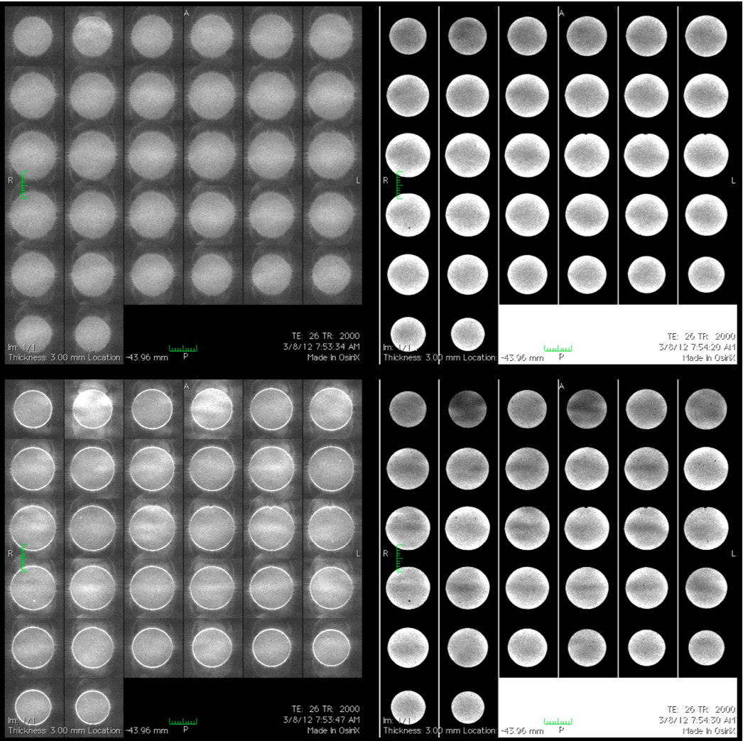
Here is a composite of summary statistical images for the control run (top row) compared to the run in which I was waggling my arms and a bottle of water inside the magnet bore (bottom row). Standard deviation images are in the left column, TSNR images on the right:

Top left: SDEV of control. Top right: TSNR of control. Bottom left: SDEV of movement during and after ACS. Bottom right: TSNR of movement during and after ACS. (Click to enlarge.)

The artifacts due to my movements are quite obvious. But, what is the cause? Was it the movement during the ACS or after the ACS that is causing the problem, or both?

Next, I repeated the movement experiment but this time I remained well clear of the magnet until after the ACS had acquired. Again, I moved my arms and the bottle of water in and out of the magnet bore, simulating a fidgety subject:

Top left: SDEV of control. Top right: TSNR of control. Bottom left: SDEV of movement after ACS only. Bottom right: TSNR of movement after ACS only. (Click to enlarge.)

The artifacts are similar to the previous movement run. So it's clear that remaining still during the ACS isn't sufficient. Movement after the ACS causes B0 shifts that lead to mismatches between the ACS and the under-sampled k-space of the time series.

At this point I wanted to be sure that it was really me moving my arms and the water bottle in the magnet that was causing these effects and not something else, such as gradient heating. So I re-ran the control experiment with me standing in the magnet room, well away from the magnet. It was almost identical to the first control run that is shown in the two composite figures above. I should also point out that I didn't re-shim during this entire testing process, so the gradient heating effects really are quite benign for GRAPPA-EPI. We should be thankful for small mercies!


Phantom tests: axial slices

My next concern was whether the apparent B0 shift sensitivity was a feature of the slice direction, sagittal slices not being especially common in fMRI. So I re-ran the same three tests - a no movement control, a run where I moved my arms and the water bottle throughout the run (including during the ACS acquisition), and a third run where I was stationary during the ACS and moved only during the under-sampled time series. The results were all but identical to the previous sagittal tests:

Top left: SDEV of control. Top right: TSNR of control. Bottom left: SDEV of movement during and after ACS. Bottom right: TSNR of movement during and after ACS. (Click to enlarge.)

Top left: SDEV of control. Top right: TSNR of control. Bottom left: SDEV of movement after ACS only. Bottom right: TSNR of movement after ACS only. (Click to enlarge.)

These results aren't a surprise when one considers that the GRAPPA-accelerated phase encoding is along the anterior-posterior direction (which is gradient Y in the magnet reference frame) for both the axial and the sagittal slices, making the effects of the 12-channel head RF coil geometry (i.e. the coil's receive fields) consistent.

Finally, note that movement of my arms and the bottle during the ACS acquisition led to far worse image artifacts, and lower TSNR, than movement only during the under-sampled time series. This is entirely expected and is in agreement with my prior experience concerning direct head motion. (See the May, 2011 post.)


But what about single-shot EPI?

Let's briefly recap. Both sagittal and axial slices were found to be susceptible to B0 shifts when using GRAPPA with R=2 acceleration. These B0 shifts arise from a modulation of the main magnetic field strength/homogeneity by moving materials that have magnetic susceptibility considerably different than air. The overall interaction depends on the amount of material in the magnet, its composition, its movement extent as well as its location relative to isocenter. That's a fairly complicated dependence! Okay, but how much worse is this situation than what we might consider to be our gold standard: single-shot EPI?

Changing the on-resonance frequency and/or the shim causes problems for single-shot, unaccelerated EPI, too. It causes ghosting for a start. (See PFUFA Part Twelve and this post in the artifact recognition series.) Thus, in my final test I used the same movement paradigm, returning to the sagittal parameters I started with. I disabled GRAPPA, shortened the echo spacing from 0.8 to 0.5 ms, reduced the matrix from 96x96 to 64x64, and left all other parameters (including TE and TR) as they had been in the GRAPPA tests for sagittal slices.

As expected, waggling my arms and a water bottle during the single-shot EPI time series did cause B0 shifts:

Top left: SDEV of control. Top right: TSNR of control. Bottom left: SDEV of movement during the EPI time series. Bottom right: TSNR of movement during the EPI time series. (Click to enlarge.)

That single-shot EPIs should be sensitive to changes in B0 makes perfect sense. However, there is one important difference between the single-shot EPI data and those acquired using GRAPPA: the B0 modulation leads to simple shifts - translations - of the images, and slight increases in ghosting, but there are no image reconstruction artifacts like the residual aliasing seen in GRAPPA-EPI.


A summary of findings

So, what did I learn? I was able to show that GRAPPA is particularly sensitive to B0 shifts that can arise from movements of a subject's body inside the magnet. It's not only direct head (or sample) movement that can cause problems and lead to image artifacts. Of course, I can't be 100% sure that it was body movements that caused the issues in the subject data I started this post with, but the effects in the phantom tests are remarkably consistent with the subject data.

What all this tells me is that motion of any sort - perhaps even breathing - during the ACS is liable to cause reconstruction errors for GRAPPA-EPI. As I mentioned in a previous post (see Note 3 of the May, 2011 post), one tactic is to have subjects swallow immediately before starting a GRAPPA-EPI acquisition, and ensure the subject doesn't move at all until after the ACS have acquired. But I'm also not thrilled by the prospects of image artifacts arising from a mismatch of the under-sampled time series and the ACS data.


When might GRAPPA be employed for fMRI?

For me, the issue of whether or not to use GRAPPA for fMRI comes down to a risk-benefit analysis. There needs to be a compelling need to either increase the spatial-temporal resolution or decrease the inherent distortion compared to standard EPI before it's worth taking the risk. You should carefully evaluate your needs, then consider alternative approaches to achieving the particular specification that might be tempting you to use GRAPPA. For example, if your particular neuroscience question doesn't require high spatial resolution and you're smoothing with a 6 mm kernel anyway, why would you use anything but single-shot EPI?

Then there is the issue of the subjects you intend to study. You might be able to make a case for adopting the higher motion sensitivity of GRAPPA if your subjects are experienced and not prone to fidgeting. If you're doing vision science and scanning only expert fMRI subjects then you might get away with the higher motion sensitivity. However, scanning children, Parkinson's disease patients and other movement-prone subjects with GRAPPA is almost certainly not advised! I would even want to test carefully before using button response boxes.

Regardless of the subjects you're studying, if you opt for GRAPPA-EPI for fMRI then you should probably try to limit all subject motion during acquisitions. There's not much you can do about subjects' breathing. But you can pay attention to comfort so that they don't want to move as much to relieve pressure points. You might be able to train them to adjust/scratch/cough/swallow only between scans.

Lest you think I'm singling out GRAPPA for unfair treatment, I should like to point out that all the parallel imaging methods currently available commercially are likely to suffer similar types of motion sensitivity for fMRI, at least as far as the "mismatch problem" is concerned. None of the popular methods - SENSE, mSENSE, GRAPPA - is truly "autocalibrating," meaning that each one of them requires some sort of reference scan in order to complete the image reconstruction. By definition, the reference scan happens at a different time to the under-sampled time series. (Usually the reference data are collected at the start of the run.) Thus, in principle, the mismatch potential exists for all parallel imaging methods in general use today. All that truly differs is the actual manifestation of motion contamination in the image data, and the effects on TSNR. For sure, some methods will be worse than others, but it seems likely that all of them would be more motion-sensitive than single-shot, unaccelerated EPI. I can't tell you anything more specific than that right now.

Of course, there are situations when the drive to use parallel imaging for fMRI might become persuasive. When thermal noise is limiting, as is the case for very high spatial resolution (2 mm voxels and below) (1,2), there might be a need to employ parallel imaging to get any signal in an image whatsoever. GRAPPA has been used as a component of super-fast imaging of the type developed using multi-band sequential echo (3) and echo volumar imaging (4,5) sequences. In these instances, not using GRAPPA would have resulted in echo train lengths that would have driven the signal into the noise, not to mention the increased distortion levels (although distortion is usually the secondary consideration, after getting the echo train length to be commensurate with the signal available via the local T2*). Still, the motion sensitivity can't be overlooked.


Final thoughts

Until someone can show me differently, my stance is as follows: GRAPPA-EPI has excessive motion sensitivity for routine fMRI use and should be avoided without careful evaluation, including piloting. Even then, I would urge you to consider every possible alternative before taking the plunge. There might be situations when a combination of careful experimental technique, high spatial resolution, particular tasks, etc. might prove better for GRAPPA-EPI than single-shot EPI or some other pulse sequence option. But you should only proceed with extreme caution.

_________________

References:

1.  C Triantafyllou, JR Polimeni & LL Wald. "Physiological noise and signal-to-noise ratio in fMRI with multi-channel array coils." NeuroImage 55, 597-606 (2011).

2.  D Mintzopolous, et al. "fMRI using GRAPPA EPI with high spatial resolution improves BOLD signal detection at 3 T." Open Magn. Reson. J. 2, 57-70 (2009).

3.  DA Feinberg, et al. "Multiplexed echo planar imaging for sub-second whole brain fMRI and fast diffusion imaging." PLoS ONE 5(12), e15710 (2010).

4.  S Posse, et al. "Enhancement of temporal resolution and BOLD sensitivity in real-time fMRI using multi-slab echo volumar imaging." NeuroImage ePub: http://dx.doi.org/10.1016/j.neuroimage.2012.02.059

5.  O Afacan, et al. "Rapid full-brain fMRI with an accelerated multi shot 3D EPI sequence using both UNFOLD and GRAPPA." Magn. Reson. Med. ePub (2011).