Impressively rapid follow-ups to a published fMRI study

Alternative post title: Why blogs can be seriously useful in research.


Last week there was quite a lot of attention to an article published in PNAS by Aharoni et al. In their study they claimed that fMRI could be useful in predicting the likelihood of rearrest in a group of convicts up for parole:

"Identification of factors that predict recurrent antisocial behavior is integral to the social sciences, criminal justice procedures, and the effective treatment of high-risk individuals. Here we show that error-related brain activity elicited during performance of an inhibitory task prospectively predicted subsequent rearrest among adult offenders within 4 y of release (N = 96). The odds that an offender with relatively low anterior cingulate activity would be rearrested were approximately double that of an offender with high activity in this region, holding constant other observed risk factors. These results suggest a potential neurocognitive biomarker for persistent antisocial behavior."

The senior author, Kent Kiehl, was interviewed on National Public Radio on Friday morning. I heard it on my way into work. An NPR interview would suggest the media attention was widespread, although I haven't looked at this aspect specifically.

What I did notice, however, was that The Neurocritic came out with two quick posts (here and here) wherein he brought up a couple of interesting limitations of the study and even ran his own re-analysis of the data, the PNAS authors having been kind enough to make their data available publicly.

This afternoon, Russ Poldrack has followed up with his own analysis and interpretation of the study's data. I'll be honest, all the stats leaves me flat-footed. But I am very seriously impressed by the way the blogosphere, combined with shared data, has been able to poke and prod the original study's conclusions.

Why am I so enthused? Because the mainstream media (still) has the power to dominate the narrative in the public sphere, and it is especially important that specific criticisms can be leveled within the same news cycle, while the public might still be paying attention to the story. So, while I think it's highly unlikely that NPR will interview the senior author of the next study that finds there is no predictive use of fMRI for recidivism - we seem to have a serious positive results bias in science - maybe there's a slim chance that NPR will interview Russ about his follow-up analysis, just to balance the record. And if not, at least those in the field have the benefit of the post-publication peer review that blogs can offer.

Quick update for Siemens users

Apologies for the lengthy absence. Many irons in the fire, etc. So until I can provide a more considered post I give you these three random tidbits:

1. Syngo MR version D13 for Verio and Skyra

There is an EPI sequence in VD13 that has a real time update of the on-resonance frequency, i.e. one that is computed and applied TR by TR, to combat drift caused by gradient heating. There are apparently versions for fMRI and diffusion-weighted imaging. I don't have any detailed information but if you are working on a Verio or a Skyra it might be time to talk to your physicist and/or local Siemens rep.

2. Phase encode direction for axial and axial-oblique EPI

Siemens uses A-P phase encoding by default whereas GE uses P-A by default. Essentially, for axial (and axial oblique) EPI the A-P direction compresses the frontal lobe but stretches occipital lobe whereas P-A stretches frontal lobe and compresses occipital. Pick your poison. (See Note 1.) Test each one out by setting the Phase enc. dir. parameter on the Routine tab. To set P-A from A-P (default) first click the three dots (...) to the right of the parameter field and open the dialog box, then enter 180 <return> instead of 0. You will probably find that the parameter change doesn't "stick" for appended scans, so saving a modified protocol in the Exam Explorer is a way to ensure the default (A-P) doesn't get reinstated without you noticing. More details to come in the next version of my user training/FAQ document.

3. Another way to force a re-shim

In my last user training/FAQ document (and here) I gave a simple way to force the scanner to re-shim at any point, e.g. when you know or strongly suspect the subject may have moved, or between lengthy blocks as a way to maintain high quality data in spite of slow subject motion and scanner drifts. But there is another way to do it and from some basic tests it looks to be superior. Here's a shaky video of the procedure conducted on a Trio running Syngo MR B17 (see Note 2):

(The essential procedure is the same for later software versions, but the layout of the 3D Shim window is slightly different.)

A checklist for fMRI acquisition methods reporting in the literature

This post updates the draft checklist that was presented back in October. Thanks to all who provided feedback. The updated checklist, denoted version 1.1, incorporates a lot of the suggestions made previously. The main difference is the reduction from three to two categories. The logic is that we should be encouraging reporting of "All of Essential plus any of Supplemental" parameters in the methods section of any fMRI publication.

(Click to enlarge.)

Explanatory notes, consolidated from the post on the draft list, and abbreviations appear below.

Inadequate fat suppression for diffusion imaging

Diffusion imaging is often included as a component of functional neuroimaging protocols these days. While fMRI examines functional changes on the timescale of seconds to minutes, diffusion imaging is able to detect changes over weeks to years. Furthermore, there may be complimentary information from the white matter connectivity obtainable from diffusion imaging – that is, from tractography - and the functional connectivity of gray matter regions that can be derived from resting state or task-based fMRI experiments.

I was recently made aware of some artifacts on diffusion-weighted EPI scans acquired on a colleagues’ scanner. When I was able to replicate the issue on my own scanner, and even make the problem worse, it was time to do a serious investigation. The origin of the problem was finally confirmed after exhaustive checks involving the assistance of several engineers and scientists from Siemens. The conclusion isn't exactly a major surprise: fat suppression for diffusion-weighted imaging of brain is often insufficient. And it seems that although the need for good fat suppression is well known amongst physics types, it’s not common knowledge in the neuroscience community. What’s more, the definition of “sufficient” may vary from experiment to experiment and it may well be that numerous centers are unaware that they may have a problem.

Let’s start out by assessing a bad example of the problem. The diffusion-weighted images you’re about to see were acquired from a typical volunteer on a Siemens TIM/Trio using a 32-channel receive-only head coil, with b=3000 s/mm² (see Note 1), 2 mm isotropic voxels, and GRAPPA with twofold (R=2) acceleration. These are three successive axial slices:

(Click to enlarge.)

The blue arrows mark hypointense artifacts whereas the orange arrow picks out a hyperintense artifact. Even my knowledge of neuroanatomy is sufficient to recognize that these crescents are not brain structures. They are actually fat signals, shifted up in the image plane from the scalp tissue at the back of the head. (If you look carefully you may be able to trace the entire outline of the scalp, including fat from around the eye sockets, all displaced anterior by a fixed amount.) I’ll discuss the mechanism later on, but at this point I’ll note that the two principal concerns are the b value (of 3000 s/mm²) and the use of a 32-channel array coil. GRAPPA isn’t a prime suspect for once!

Now, part of the problem is that the intensity of the artifacts – but not their location - changes as the direction of the diffusion-weighting gradients changes. In the following video you see the diffusion-weighted images as the diffusion gradient orientation is changed through thirty-two directions (see Note 2):

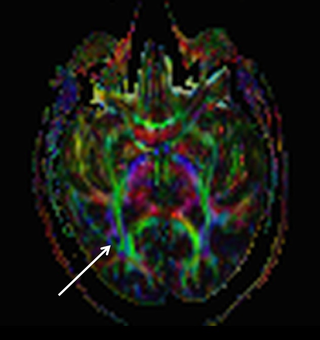
The signal from white matter fibers changes as the diffusion gradient direction changes. That’s what you want to happen. But the displaced fat artifacts also change intensity with diffusion gradient direction, meaning that the artifact is erroneously encoded as regions of anisotropic diffusion. Thus, when one computes the final diffusion model, the brain regions contaminated by fat artifacts end up looking like white matter tracts. In the next figure the data shown above was fit to a simple tensor model, from which a color-coded anisotropy map can be obtained:

The white arrow picks out the false “tract” corresponding to the artifact signal crescent we saw on the raw diffusion-weighted images. I suppose it’s remotely possible that this is the iTract, a new fasciculus that has evolved to connect the subject’s ear to his smart phone, but my money is on the fat artifact explanation.

Clearly, in the above image there is no easy way to distinguish the artifact from real white matter tracts by eye, except by using your prior anatomical knowledge. And it's likely to confuse tractographic methods, too, because it has very similar geometric properties to those that tractographic methods attempt to trace. So let's take a look at the origin of the problem and then we can get into what you want: solutions. 

Review: Differentiating BOLD from non-BOLD signals in fMRI time series using multi-echo EPI

Disclaimer: I'm afraid I haven't done a very good job reviewing the entirety of this paper because the stats/processing part was pretty much opaque to me. I've done my best to glean what I can out of it, and then I've focused as much as I can on the acquisition, since that is one part where I can penetrate the text and offer some useful commentary. Perhaps someone with better knowledge of stats/ICA/processing will review those sections elsewhere.


The last paper I reviewed used a bias field map to attempt to correct for some of the effects of subject motion in time series EPI. A different approach is taken by Prantik Kundu et al. in another recently published study. In their paper, Differentiating BOLD from non-BOLD signals in fMRI time series using multi-echo EPI, Kundu et al. set out to differentiate between signal changes that have a plausible neurally-driven BOLD origin from those that are likely to have been modulated by something other than neuronal activity. In the latter category we have cardiac and respiratory fluctuations and, of course, subject motion.

The method involves sorting BOLD-like from spurious changes using an independent component analysis (ICA) and to then "de-noise" the time series before applying connectivity analysis. For resting state fMRI in particular, the lack of any sort of ground truth and an absence of independent knowledge that one has with task-based fMRI makes disambiguating neurally driven signal changes from artifacts a major problem. Kundu et al. use a relatively simple philosophical approach to the separation:

"We hypothesized that if TE-dependence could be used to differentiate BOLD and non-BOLD signals, non-BOLD signal could be removed to denoise data without conventional noise modeling. To test this hypothesis, whole brain multi-echo data were acquired at 3 TEs and decomposed with Independent Components Analysis (ICA) after spatially concatenating data across space and TE. Components were analyzed for the degree to which their signal changes fit models for R₂* and S₀ change, and summary scores were developed to characterize each component as BOLD-like or not BOLD-like."

And, noting again the caveat that there is an absence of ground truth, the approach seems to work:

"These scores clearly differentiated BOLD-like “functional network” components from non BOLD-like components related to motion, pulsatility, and other nuisance effects. Using non BOLD-like component time courses as noise regressors dramatically improved seed-based correlation mapping by reducing the effects of high and low frequency non-BOLD fluctuations."

Review: Using a bias field map to improve motion correction of EPI time series

In a new paper entitled "Effects of image contrast on functional MRI image registration," Gonzalez-Castillo et al. evaluate the performance of motion correction (a.k.a. registration) following a pre-processing step that aims to remove the contrast imparted across images due to receive (and/or transmit) field heterogeneity. A bias field map is estimated from a target EPI, and this reference image is then used to normalize the other images in the time series. There are other aims in the paper, too: specifically, to evaluate the performance of image registration (EPI to EPI, or EPI to MP-RAGE anatomical) when the T1 contrast of time series EPIs is altered via the excitation RF flip angle. But in this post I am going to focus on the normalization part because it involves the RF receive field heterogeneity, and this instrumentally-induced contrast is of particular concern for exacerbating motion sensitivity in fMRI (as explained here).

Although others have compared prescan normalization between different array coils (see the references in this paper), this is the first paper I've seen that compares motion correction performance for EPI time series acquired with an array coil (a 16-channel array) to a single channel birdcage coil. Now, this isn't quite the straightforward comparison I might like - with the receive fields being the only difference - because in this instance the birdcage is also used to transmit the excitation RF pulses, making the transmission (Tx) field for the birdcage experiment more spatially heterogeneous than will be produced from the body RF coil that's used when acquiring with a receive-only array coil. Following? In other words, for the 16-channel array the receive (Rx) field heterogeneity is likely to dominate whereas for the birdcage coil the heterogeneities of both the transmit and receive fields are salient. Still, it's worth a look since the coil comparison highlights the issue of the scanner hardware's influence on EPI contrast, and on subsequent motion correction.

Motion problems in fMRI: Receive field contrast effects

Motion has been identified as a pernicious artifact in resting-state connectivity studies in particular. What part might the scanner hardware play in exacerbating the effects of subject motion?

My colleague over at MathematiCal Neuroimaging has been busy doing simulations of the interaction between the image contrast imposed by the receiver coil (the so-called "head coil") and motion of a sample (the head) inside that coil. The effects are striking. Typical amounts of motion create signal amplitude changes that easily rival the BOLD signal changes, and spurious spatial correlations can be introduced in a time series of simulated data.

The issue of receive field contrast was recognized in a recent review article by Larry Wald:

"Highly parallel array coils and accelerated imaging cause some problems as well as the benefits discussed above. The most problematic issue is the increased sensitivity to motion. Part of the problem arises from the use of reference data or coil sensitivity maps taken at the beginning of the scan. Movement then leads to changing levels of residual aliasing in the time-series. A second issue derives from the spatially varying signal levels present in an array coil image. Even after perfect rigid-body alignment (motion correction), the signal time-course in a given brain structure will be modulated by the motion of that structure through the steep sensitivity gradient. Motion correction (prospective or retrospective) brings brain structures into alignment across the time-series but does not alter their intensity changes incurred from moving through the coil profiles of the fixed-position coils. This effect can be partially removed by regression of the residuals of the motion parameters; a step that has been shown to be very successful in removing nuisance variance in ultra-high field array coil data (Hutton et al., 2011). An improved strategy might be to model and remove the expected nuisance intensity changes using the motion parameters and the coil sensitivity map."

In our recent work we take a first step towards understanding the rank importance of the receive field contrast as it may introduce spurious correlations in fMRI data. It's early days, there are more simulations ongoing, and at this point we don't have much of anything to offer by way of solutions. But, as a first step we are able to show that receive field contrast is ignored at our peril. With luck, improved definition of the problem will lead to clever ways to separate instrumental effects from truly biological ones.

Anyway, if you're doing connectivity analysis or otherwise have an interest in resting-state fMRI in general, take a read of MathematiCal Neuroimaging's latest blog post and then peruse the paper submitted to arXiv, abstract below.

____________________

A Simulation of the Effects of Receive Field Contrast on Motion-Corrected EPI Time Series

D. Sheltraw, B. Inglis

(Submitted on 12 Oct 2012)

The receive field of MRI imparts an image contrast which is spatially fixed relative to the receive coil. If motion correction is used to correct subject motion occurring during an EPI time series then the receiver contrast will effectively move relative to the subject and produce temporal modulations in the image amplitude. This effect, which we will call the RFC-MoCo effect, may have consequences in the analysis and interpretation of fMRI results. There are many potential causes of motion-related noise and systematic error in EPI time series and isolating the RFC-MoCo effect would be difficult. Therefore, we have undertaken a simulation of this effect to better understand its severity. The simulations examine this effect for a receive-only single-channel 16-leg birdcage coil and a receive-only 12-channel phased array. In particular we study: (1) The effect size; (2) Its consequences to the temporal correlations between signals arising at different spatial locations (spatial-temporal correlations) as is often calculated in resting state fMRI analyses; and (3) Its impact on the temporal signal-to-noise ratio of an EPI time series. We find that signal changes arising from the RFC-MoCo effect are likely to compete with BOLD (blood-oxygen-level-dependent) signal changes in the presence of significant motion, even under the assumption of perfect motion correction. Consequently, we find that the RFC-MoCo effect may lead to spurious temporal correlations across the image space, and that temporal SNR may be degraded with increasing motion.